Hi all – this is a little webpage about my upcoming visit to Imperial in Feb 2018. If you  have any questions in advance feel free to message me!

Why am I visiting? 

While I’m at Imperial, I’ll be giving a talk on my research in lithosphere deformation – it will have a title something like Deformation driven by deep and distant structures: influence of mantle lithosphere scarring in crustal tectonics. I’ll be presenting numerical modelling results using a numerical code called ASPECT.  The code is a relatively new venture with quite big ideas about itself – which is the other reason why I am visiting. I’m keen to chat to the group to see if ASPECT could be used to supplement any existing studies/research programs. A main point of ASPECT is to be usable and extendible – I think it could be a great tool for the group at Imperial.

Examples of code output

Finite element mesh, velocity, viscosity and strain rate fields in the case of extensional boundary conditions (top) and compressive boundary conditions (bottom) at t=500kyr.

Panel (a) shows an equatorial cross section of the temperature distribution and resulting flow from a harmonic perturbation. Panel (b) shows the resulting geoid, and panels (c) and (d) show the resulting surface and bottom topography. Note that we have subtracted the mean surface and bottom topography in the respective panels (c and d) as a postprocessing step outside of Aspect.

Strain rate and compositional field after 5e6 years of extension. The black line marks the 550 ◦C isotherm.

Strain rate(s−1) after 10e6 years of extension of cookbook example. The black line marks the 550 ◦C isotherm. The numerical resolution is (1 km)

Panels (a) and (b) show the density distribution as prescribed from the shear wave velocity model S20RTS and the resulting flow for a global refinement of 4. This model assumes a constant scaling between shear wave and density perturbations. Panel (c) shows the great circle (dashed blue line) along which the top slices are evaluated. Panels (c) and (d) show the resulting heat flux density for a global refinement of 2 (c, cookbook) and 4 (d). The colorbar ranges from 13 to 19 mW/m2 for panel (c) and from 35 to 95 mW/m2 for panel (d).

3D crustal modelling in extension. Finite element mesh, velocity, viscosity and strain rate fields at the end of the first time step after one level of strain rate-based adaptive mesh refinement.

Convection in a spherical shell: Snapshot of isosurfaces of the temperature field at time t ≈ 1.06 · 109 years with a quarter of the geometry cut away. The surface shows vectors indicating the flow velocity and direction.

Simple convection in a quarter of an annulus: Snapshots of the temperature field at times t = 0, t = 1.2 · 107 years (time step 2135), and t = 109 years (time step 25,662). The bottom right part of each figure shows an overlay of the mesh used during that time step.

The first row of this figure shows the surface dynamic topography resulting from the flow of a seismic input for a global refinement of 2 (a, cookbook) and 4 (b). The colorbar ranges from -2400m to 400m for panel (a) and from -2000m to 1600m for panel (b). The second row shows the dynamic topography at the core mantle boundary for the same model and a refinement of 2 (c, cookbook) and 4 (d). Averages of the dynamic topography fields are indicated at the bottom left of each panel. The bottom row shows the geoid anomalies from this model at the surface for refinement of 2 (e, cookbook) and 4 (f).

Cross sections of the present-day state showing the sublithospheric flow channel from the Réunion plume along the Rodrigues Ridge toward the Central Indian Ridge (CIR) in (a) model PlumePosVar9 and (b) model NoGlobalFlow, slightly shifted to the south to cut through the plume conduit. Colors show the excess temperature relative to the adiabat and the area exceeding 5% melt fraction, respectively. The dark red contour outlines the plume and the white contour the base of the lithosphere. Orange arrows depict the global flow, green arrows the plate motions. The inset map shows the position of the cross section in a top view of the model.

Global mantle convection models with paleo subduction history. Final state of a global mantle convection simulation after 250 Ma of model time. Top panels: Isosurfaces of −150 K (white to blue) and +300 K (rainbow coloured) temperature deviation from an adiabatic temperature profile for the African hemisphere (left) and the Pacific hemisphere (right). Colours visualize height above the core–mantle boundary, and coastlines are shown in black outlines. Bottom panels: Equatorial slices through the model showing temperature deviation and finite-element mesh (centre left) and viscosity (centre right).In all slices the Greenwich meridian is ‘up’ and the view is directed from the North pole to the South pole.

Subduction model. Strain rate field over time together with subjecting plate and oceanic plate isocontours. Also shown is the adaptive mesh following the subducting plate into the mantle.

A bit about the code 

ASPECT stands for: Advanced Solver for Problems in Earth’s ConvecTion

It is written in a purposely extendible fashion, meaning it can be easily built on by different groups around the world – each adding something new and exciting to the code (which is written in C++).

It was built to support research in simulating convection in the Earth’s mantle and elsewhere. However, the latter part of the sentence is slightly misleading – as it sounds like it is only a code for mantle convection. ASPECT can also be used to simulate of lithosphere deformation (which is what I use it for).

The code generally runs on a supercomputer, but smaller simulations can be run on a desktop or even a laptop.

Community driven 

The code is free and developed out in the open (here, to be exact, so you can see what people are working on and what bugs there are). A big feature of ASPECT is that it is science-driven in it’s development – meaning that if lots of people are interested in developing rifting models or salt tectonic simulations, the code will be steered to incorporate all the nuanced parameters required. From the website:

It has grown from a pure mantle-convection code into a tool for many geodynamic applications including applications for inner core convection, lithospheric scale deformation, two-phase flow, and numerical methods development….

And it is still developing, it is not finished, and has a long way to go!

Another plus is that there is a pretty good mailing list. This sounds boring but it is really good – it is a venue for users to share problems and issues in the hope that other members of the community have either seen them and solved them, or can give advice on how to fix it.

Different scales

You a fan of 2D? Or 3D better? ASPECT is built to extend a model dimensionally without too much difficultly.

What do you want to model – pick a geometry that is already built into the code: Box, box with lithosphere boundary conditions, chunk, ellipsoidal chunk, sphere, spherical shell, or unspecified!

Usable, Adaptable, and Extendable

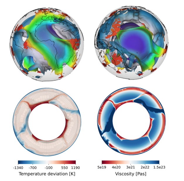
The beauty of the code is that you can throw a lot at it. One example is apply seismic input to generate flow fields, to generate topography:

Basic setups as a starting point

At present, there are 30+ ‘cookbook’ examples that are available to use once the code is installed. Examples of interest include:

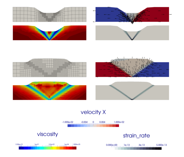
• 2D crustal model and 3D crustal model (as shown above)
• continental extension model (shown below)
• flow field and dynamic topography generation from seismic input
• prescribed plate boundary motion

The input files for these codes are easy to understand, and easy to change. I will go through the input file for the continental extension cookbook when I am visiting, as I think it will be a good starting point.

As described in the file – the cookbook is based off numerous published studies, including

• Brune, S., Heine, C., Perez-Gussinye, M., and Sobolev, S.V. (2014), Nat. Comm., v.5, n.4014, Rift migration explains continental margin asymmetry and crustal hyperextension
• Huismans, R., and Beaumont, C. (2011), Nature, v.473, p.71-75.
• Naliboff, J., and Buiter, S.H. (2015), Earth Planet. Sci. Lett., v.421, p.58-67

All these parameters can be modified easily by the user. Below are example of this input file that is ‘out of the box’ ready to use:

A low resolution video of the model can be seen below.

What is important: This starting input file can be quickly extended to 3D, increased in depth, and have the rheology changed.

Examples of published studies with ASPECT

Glerum et al. (2018) – Implementing nonlinear viscoplasticity in ASPECT: benchmarking and applications to 3D subduction modeling Solid Earth

Bredow et al. (2017) – How plume-ridge interaction shapes the crustal thickness pattern of the Réunion hotspot track G-cubed

Heister et al. (2017) High accuracy mantle convection simulation through modern numerical methods – II: realistic models and problems Geophysical Journal International

Gassmoeller et al. (2016) – Major influence of plume-ridge interaction, lithosphere thickness variations, and global mantle flow on hotspot volcanism-The example of Tristan G-cubed

Video caption: (top) Plume position, lithosphere thickness, topography; 
(bottom) plume position, melt fraction, crust thickness for evolution of Tristan plume-ridge interaction (140 Ma to present)

Downsides

It can be a bit of a pain to install, but with people on hand it can be simple. I’m available to help with installation and to create an installation guide – like the ones I’ve previously created. Another downside is that the code can take a little while to complete simulations.

A bit more about the code (links) 

https://aspect.geodynamics.org  – the software page.

Join the mailing list here! – it is an excellent way to get involved with the development and to voice questions.

Publications using ASPECT  – from the software page.

https://github.com/geodynamics/aspect – GitHub development page that has a wiki page on installation (https://github.com/geodynamics/aspect/wiki)

ASPECT User Manual  – updated regularly (currently 30 MB and 454 pages).

ASPECT CIG Community page (overview) and ASPECT CIG Wiki page (slightly dated).

2014 Introduction to ASPECT powerpoint presentation

From the website:

ASPECT is a code to simulate problems in thermal convection. Its primary focus is on the simulation of processes in the earth’s mantle, but its design is more general than that. The primary aims developing ASPECT are:

• Usability and extensibility: Simulating mantle convection is a difficult problem characterized not only by complicated and nonlinear material models but, more generally, by a lack of understanding which parts of a much more complicated model are really necessary to simulate the defining features of the problem. This uncertainty requires a code that is easy to extend by users to support the community in determining what the essential features of convection in the earth’s mantle are.
• Modern numerical methods: We build ASPECT on numerical methods that are at the forefront of research in all areas — adaptive mesh refinement, linear and nonlinear solvers, stabilization of transport-dominated processes. This implies complexity in our algorithms, but also guarantees highly accurate solutions while remaining efficient in the number of unknowns and with CPU and memory resources.
• Parallelism: Many convection processes of interest are characterized by small features in large domains — for example, mantle plumes of a few tens of kilometers diameter in a mantle almost 3,000 km deep. Such problems require hundreds or thousands of processors to work together. ASPECT is designed from the start to support this level of parallelism.
• Building on others’ work: Building a code that satisfies above criteria from scratch would likely require several 100,000 lines of code. This is outside what any one group can achieve on academic time scales. Fortunately, most of the functionality we need is already available in the form of widely used, actively maintained, and well tested and documented libraries. Thus, ASPECT builds immediately on top of the deal.II library for everything that has to do with finite elements, geometries, meshes, etc.; and, through deal.II on Trilinos for parallel linear algebra and on p4est for parallel mesh handling.
• Community: We believe that a large project like ASPECT can only be successful as a community project. Every contribution is welcome and we want to help you so we can improve ASPECT together.